
Antikythera Equation of Time Correction
Earth’s Eccentricity
The effect of Earth’s eccentricity is very similar to the lunar anomaly pin-slot system, it is due to the difference in eccentric anomaly and mean anomaly. In other words, the speeding up of the planet at the lowest point in its orbit (perihelion) and the slowing down of the planet at the highest point in its orbit (aphelion). The magnitude of this effect is only dependent on the eccentricity of the orbit: for Earth the eccentricity is 0.017 and thus the maximum error (via Kepler’s Equation) is 1.92 deg or 7.66 min. It has a period of one earth year and is phased such that error is zero at aphelion and perihelion.
Earth’s Axial Tilt
This effect is less intuitive to visualize than the former, but is a result of the sun’s path through the celestial sphere. Since the axis of rotation of the earth is tilted (but stays roughly fixed relative to the stars) the height of the sun’s path off of the horizon (the ecliptic) varies throughout the year. The celestial sphere is mapped using right ascension, similar to longitude on earth, and declination, similar to latitude. As such, only right ascension visually changes over time as the earth rotates, while the declination remains fixed. Since the sun’s path through the sky is moving the component in the right ascension direction varies, so even if the sun moved at a constant rate the varying component in right ascension would yield a varying effect. The maximum error as a result of this effect is 2.47 deg or 9.87 minutes. This occurs with a period of half of a year and is phased such that error is zero at the equinoxes and solstices.
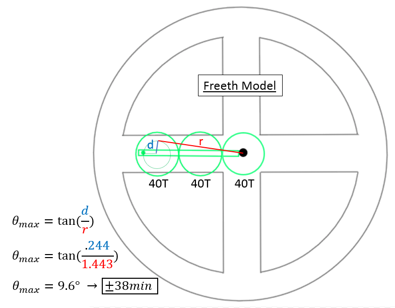
The Historical Mechanism
The original Antikythera Mechanism (AM) is believed to have has a correction for the difference between the apparent sun position and the mean sun, although in a more simplistic manner than we know it now. At the time, this difference (which we now call the equation of time) was known to exist but had not been refined beyond a simple oscillation similar to the lunar anomaly or a planet’s retrograde motion. As such, it is justified that both the Freeth and Wright models of the AM use the same pin-in-slot pointer mechanism as the inferior planet assemblies. The magnitude of the correction is fairly large but also consistent with the estimate of the approximate time period: two centuries later Book III of Ptolemy’s Almagest states the maximum correction as 5/9ths of an hour (33 min) which appears very close to the Freeth dimensions.

Constructing a Mechanical Representation
The equation of time is simply two sinusoidal signals added together, so there is good potential to emulate it using a mechanical assembly. For several excellent examples of how this can be done I would recommend the animations at equation-of-time.info. There are several ways to combine scotch yokes and epicyclic gears to resolve the rotational motion into linear without incurring cosine errors, but for the purposes of the AM reproduction these were deemed too complex compared to a whippletree.
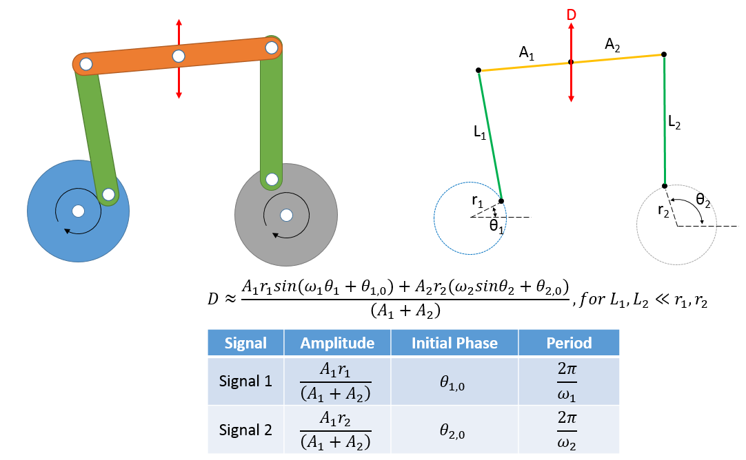
Basic Geometry
A whippletree is typically used to equalize forces, for example ensuring that a team of draft horses are all seeing equal loading when pulling a plow, but it can also be used as a signal combiner. In the image to the right this is laid out geometrically, in the simplest incarnation. Note that there is a built in small-angle approximation and as the two L’s get shorter compared to the r’s this model will degrade. Still, it is a useful starting point. We know the period of both the eccentricity and the axial tilt terms to be 1 year and 1/2 year respectively. The input to the gear train is a 40T gear rotating at a 1 year period, so this is easily accomplished with a 40T and 20T gear. The amplitudes are chosen based on the maximum errors of the two effect relative to the main leg length (red in image).

The Equation of Time
The equation of time is now understood to be not a single oscillating correction, but rather the summation of two oscillating effects: Earth’s eccentricity and the tilt of its axis. Together, these two effects create a distinct dual sinusoidal curve.
Resultant Motion Using Basic Definition
The mechanism when constructed using this simple geometric definition does show a visibly similar output, but the sizing of the gears is such that the assumption used (L’s>>r’s) is rather poor.

Improvement Using an Optimization Program
To address this and reduce the error, an optimization algorithm was used to vary the geometry slightly (L1, L2, r1, r2, main leg length, A1, A2, and A1/A2 cross dimension) and minimize the difference from the true EoT curve. This was performed using fminsolve in MATLAB and resulted in the design below, which is visibly improved from the previous iteration to the point of being acceptable to incorporate into the larger Antikythera Mechanism. Note that there are additional variables, such as the phase shift between the two functions and the phase offset between the two gears, that could be utilized, however the solution attained is more than sufficient.

By: Spencer Connor
Errata: The Antikythera Mechanism shows solar motion along the ecliptic (rather than the celestial equator), and as a result only models the effect of eccentricity. The effect of obliquity comes from the reduction from the ecliptic to the celestial equator, so it is understandable that it not be included in the mechanism. I came to this realization after writing this page and apologize for any confusion
In Practice
Now let’s compare this to the as-built mechanism using motion tracking. In this case two dots of pink paint were put on the arm and a video was taken of the mechanism running being driven by a drill. In each video frame, the paint spots were identified via centroiding and an angle established between them. When this angle is analyzed across a full cycle we see the distinctive dual sinusoidal signal emerge. There are errors present, but given the reliability of the linkage set is only driven by the tolerance of the part dimensions it is far more likely that these are driven by the effects of the test setup such as variability of the drill motor speed and parallax of the camera field-of-view.